Defining custom potentials#
Custom potentials can be implemented by defining a class that inherits from either the LinearPotential or NonLinearPotential classes. In the following, we will exemplify this by implementing a simple harmonic oscillator potential, displaced from the origin:
where \(m\) is the mass, \(\omega_x\) and \(\omega_y\) the frequencies in the x and y directions, and \(x_0\) and \(y_0\) the displacements in the x and y directions. We denoted with \(X\) and \(Y\) the coordinates in SI units.
Since TorchGPE works with adimensional units, we need to divide by the unit of energy \(E_l = \hbar \omega_l = m l^2 \omega_l^2\):
where we called \(x\) and \(y\) the coordinates in adimensional units.
This is a time independent linear potential, so we will inherit from the LinearPotential class:
 1from torchgpe.utils.potentials import LinearPotential
 2
 3
 4class DisplacedTrap(LinearPotential):
 5
 6    def __init__(self, fx, fy, x0 = 0, y0 = 0):
 7        super().__init__()
 8
 9        self.fx = fx
10        self.fy = fy
11        self.x0 = x0
12        self.y0 = y0
In this first code, we just defined the class DisplacedTrap to inherit from LinearPotential. We also defined the constructor, which takes the frequencies and displacements as arguments and stores them as attributes of the class. We would like the user to express these values in SI units. For this reason, since TorchGPE works with adimensional quantities, we need to adimensionalize them before using them in the code. The frequencies can be adimensionalized by dividing them by the pulse \(\omega_l\), while the displacements should be divided by \(l\). These quantities are not provided to the potential just yet, but are stored in the Gas class. This is passed to the potential before a simulation starts via the set_gas() method.
After the gas has been provided to the potential but before the simulation starts, an additional initialization step is performed. This is done by the on_propagation_begin() function, which can be overridden in the custom potential class. In this case, we will use it to adimensionalize the frequencies. This step is also importat to allow some of the parameters to be time-dependent. In this example, we will allow the displacement to be changed in time.
 1from torchgpe.utils.potentials import LinearPotential, any_time_dependent_variable, time_dependent_variable
 2import numpy as np
 3
 4class DisplacedTrap(LinearPotential):
 5
 6    def __init__(self, fx, fy, x0 = 0, y0 = 0):
 7        super().__init__()
 8
 9        self.fx = fx
10        self.fy = fy
11        self.x0 = x0
12        self.y0 = y0
13
14    def on_propagation_begin(self):
15        self.is_time_dependent = any_time_dependent_variable(
16            self.x0, self.y0)
17
18        self._omegax = 2*np.pi * self.fx / self.gas.adim_pulse
19        self._omegay = 2*np.pi * self.fy / self.gas.adim_pulse
20
21        self._x0 = time_dependent_variable(self.x0)
22        self._y0 = time_dependent_variable(self.y0)
With these changes, we are checking the nature of x0 and y0. They can either be constants (meaning that the potential is time-independent), or functions of time. In each case, we use the time_dependent_variable() function to turn them into functions of time (if the value is a constant, the function will always return that same value). We also adimensionalize the frequencies.
Note
The time dependent variables cannot be adimensionalized at this stage, since they are not numbers, but functions. We will do this later, when we evaluate the potential.
Finally, the definition of a linear potential requires the implementation of the get_potential() method. This method takes the adimensional coordinates as arguments and returns the value of the potential at those coordinates. A time argument is also provided.
Note
In case the propagation is in imaginary time, the value of time does not have a physical meaning. Nonetheless, only time independent variables are supported by imaginary time, so the time argument will always be irrelevant.
 1from torchgpe.utils.potentials import LinearPotential, any_time_dependent_variable, time_dependent_variable
 2import numpy as np
 3
 4class DisplacedTrap(LinearPotential):
 5
 6    def __init__(self, fx, fy, x0 = 0, y0 = 0):
 7        super().__init__()
 8
 9        self.fx = fx
10        self.fy = fy
11        self.x0 = x0
12        self.y0 = y0
13
14    def on_propagation_begin(self):
15        self.is_time_dependent = any_time_dependent_variable(
16            self.x0, self.y0)
17
18        self._omegax = 2*np.pi * self.fx / self.gas.adim_pulse
19        self._omegay = 2*np.pi * self.fy / self.gas.adim_pulse
20
21        self._x0 = time_dependent_variable(self.x0)
22        self._y0 = time_dependent_variable(self.y0)
23
24    def get_potential(self, X, Y, time = None):
25        return 0.5 * ( self._omegax**2 * (X - self._x0(time)/self.gas.adim_length)**2 +
26                       self._omegay**2 * (Y - self._y0(time)/self.gas.adim_length)**2 )
Note
Note how the pulse omega has been adimensionalized already, and hence it can be used directly. The displacement, on the other hand, has to be adimensionalized at this stage, since it is a function of time.
As a first sanity check, we can compare the potential with the Trap potential implemented in TorchGPE. To do so, we set the displacement to \(0\) and the frequencies to \(400,\,\text{Hz}\). The image below shows the comparison between the two potentials.
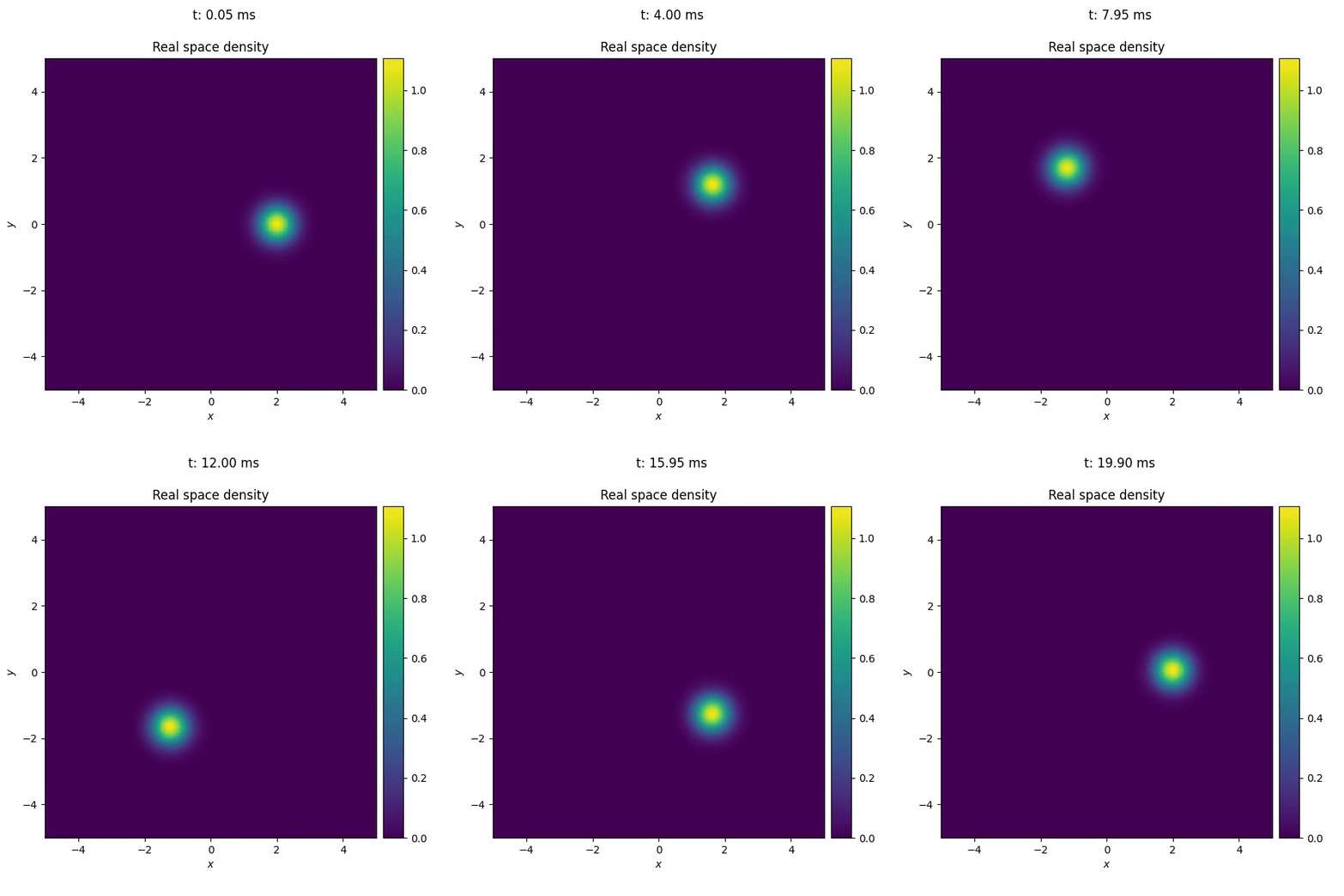
By using the propagate() function of TorchGPE, we can also test the behaviour of the potential in time. In the following example, we move the center of the trap along a circular path. By doing it slowly, the cloud adiabatically adapts to the changes in the potential; that is, the shape of the BEC remains the gaussian profile typical of the ground state of an harmonic oscillator, but its center is slowly displaced. The image below shows the result of the simulation.
